Modeling for Reinforcement Learning and Optimal Control: Double pendulum on a cart
Modeling is an integral part of engineering and probably any other domain. With the popularity of machine learning a new type of black box model in form of artificial neural networks is on the way of replacing in parts models of the traditional approaches. However we think that this does not mean that traditional models will be less significant, but they might get even more important in some domains. Traditional models can for example be used to feed the deep learning algorithms that (at the moment) are hungry for large amounts of data, by generating data using classical modeling approaches.
In the domain of control theory, Optimal Control explicitly relies on a white-box model for the dynamical system, while (model-free) Reinforcement Learning trains a black-box model without knowing the behavior of the system (or environment, or plant). The two disciplines overlap where optimal control relies on black-box model for the dynamical system, or where optimal control solutions are used to train neural networks, or where reinforcement learning depends on some kind of model (model-based reinforcement learning). We think that learning and control algorithms can be implemented most efficiently by utilizing the interplay between model-based and model-free algorithms when the computational (lookup) speed and expressive power of deep neural networks is combined with the accuracy of physical eqations that are known for many types of systems.
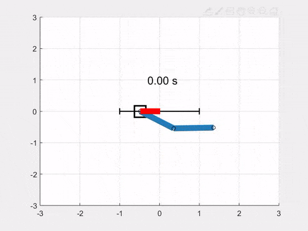
In this article we show how to implement a simulation model of a double pendulum on a cart, or double-pole cart, or double cart-pole if you like. At the end of the article we will be able to simulate the double pendulum system on a cart like this:

You will also find the link to the repository, and links to download the simulation code for Python and Matlab/Octave at the end of the article.
Basic system outline
We briefly summarize the features/requirements that we would like to implement for the model:
- The system has a cart that can move linearly along the x-axis.
- The cart can be controlled by a limited force $f$ that acts along the x-axis.
- In the center of the cart a pole/pendulum is attached by an uncontrolled revolute joint.
- At the end of the first pole, a second pole is connected to the first pole by a second uncontrolled revolute joint.
- The system should have realistic physical behavior, i.e. we use physical parameters like mass, momentum.
- We would like to be able to simulate the system from a given, or randomly chosen state $x_0$.
Here, we drew a picture of the system:
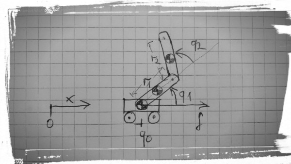
The physical properties of the double pendulum on a cart are described by a set of parameters which we choose (more or less) arbitrarily:
The state of the system
With the model equations we want to describe mathematically how the system evolves with time. But first we need to define the state of the system which describes the situation in which the system currently is. The state has to have Markov property which says something like: you should be able to predict future states, when you have only the current state given. We need this property to be able to simulate the system.
Therefore the state usually does not only include the current location or configuration of the system but also the velocity of the system. Because of Newton’s Laws we can describe the state of classical mechanical systems by its position and velocity. We know that the system continues moving when there are no forces, and it will accelerate/decelerate when there are external forces according to $F=m a$ etc.
So for our double pole cart system, we can describe the state by the following set of variables
This choice of state is a minimal representation of the state of the system. All variables are scalar, and real numbers. We do not need to describe e.g. the position of the cart in y-direction as the cart can not move upwards (only the poles).
We collect all the state variables in a column vector as
The dynamical system equations
Now follows the hard part! We use the Euler–Lagrange equations [wikipedia] to model the system dynamics. The Euler–Lagrange method is an energy based method that is a bit easier and requires less thinking than for example the (recursive) Newton-Euler method. You can apply this method quiet programmatically to many types of systems.
We start with calculating the center of mass positions of the three body parts of the cart-pole system, and express the positions as functions of the state variables. We derive the center of mass positions because we can use them to define the potential and kinetic energies of the body parts which we will use to obtain the dynamical equations. The three body parts are: the cart, the first pole, the second pole.
Kinematics The kinematics describe the static and moving structures of a system without the inertial and accelerating properties. For the double cart-pole we therefore describe the center of mass positions and velocities.
The position of the cart is easy:

as the y-coordinate of the cart is always zero.
The center of mass position of the first pole is half-way along the first pole. Here is another picture:
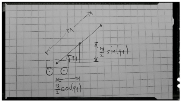
From the picture we can see that the position of the first pole can be calculated by
The center of mass position of the second pole can be derived similarly. Here we need to go to the end of the first pole (not only the half length), and add the two joint angles to get the direction of the second pole. The position of the second pole can be calculated by
From the center of mass positions we can get the velocities by differentiation. The velocity of the cart is given by

the center of mass velocity of the first pole is given by
and the velocity of the second pole is

Dynamics The dynamics of a system describe the inertial and accelerating properties of a system.
We derive the dynamics using the Euler-Lagrange energy method. We start with the kinetic energy. The overall kinetic energy is the sum of the kinetic energies of the three body parts.
The kinetic energy of the cart is

the kinetic energy of the first pole is

and the kinetic energy of the second pole is

For the potential energy of the system we again sum the potential energies of the individual parts. The cart has constant potential energy as it can not move up or down in the earth gravitational field. We can therefore omit it as it would be eliminated in the equations later.
The potential energy of the first pole is

and the potential energy of the second pole is

where p_1^y and p_2^y are the y-coordinates of the center of mass positions (the height values of the poles).
Now we can plug the kinetic energies and the potential energies into the Euler-Lagrange equation:
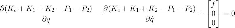
where q_0, q_1, q_2 are the coordinates of the system, \dot{q_0}, \dot{q_1}, \dot{q_2} are the velocities of the system, and $f$ is the force input (external force) that only acts on the cart in x-direction.
We can calculate the derivatives in the Euler-Lagrange equation by hand, and solve for \ddot{q}_0, \ddot{q}_1, \ddot{q}_2 but it is easier and less error prone to let the computer do the calculations for you. We prepared scripts in Python and Matlab for you that use symbolic toolboxes with symbolic differentiation and do the calculation for us. From the scripts it turns out that we get something a bit more complicated than we expected! So here it comes..
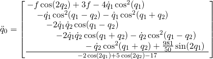
Ok we give up here writing down all the equations …
These type of equations are called ordinary differential equations as they relate the state variables q_0, q_1,q_2, \dot{q}_0, \dot{q}_1, \dot{q}_2 to their derivative \ddot{q}_0, \ddot{q}_1, \ddot{q}_2. Remember that our state was given by
We can now use a numerical integration method like explicit Euler [wikipedia], Runge-Kutta 4 [wikipedia], or even implicit methods like implicit Euler [wikipedia], BDF [wikipedia], or Collocation [wikipedia] to simulate the system. Fortunately in Python and Matlab there are already excellent implementation available that we can use (although at least the explicit methods are super easy to implement!).
To be able to use the integration methods in Matlab and Python have to define a ordinary differential equation function $f(x)$ which maps the state variables $x$ to the time derivative of the state $\dot{x}$:

which for the double pendulum system is
for the state x, \ddot{q}_0, \ddot{q}_1, \ddot{q}_2 are given by the long equations from above, and the control input f that appears in the equations can be assumed given, as we are just simulating the system. The upcoming articles will cover how to determine the control input by either Reinforcement Learning or Optimal Control.
Simulation code
And here are the Python and Matlab implementations to simulate the system starting from a random state $x_0$ for 8 seconds.
Python:
import numpy as np
import math
from scipy.integrate import solve_ivp

def main():
  # get a random starting state between min state and max state
  x_min = np.array([-1, -np.pi, -np.pi, -.05, -1, -1]);
  x_max = -x_min;
  x0 = np.random.uniform(low=0.0, high=1.0, size=6) * \
       (x_max-x_min)+x_min;

  # simulate
  t_eval = np.arange(0, 8, 0.025);
  sol = solve_ivp(dpc_ode, [0,8], x0, method="RK45", t_eval=t_eval);

def dpc_ode(t, x):
  q_0 = x[0];
  q_1 = x[1];
  q_2 = x[2];

  qdot_0 = x[3];
  qdot_1 = x[4];
  qdot_2 = x[5];
  f = 0;

  qddot_0 = (4.0*f*math.cos(2.0*q_2)-6.0*f+
             4.0*qdot_1**2*math.cos(q_1)+
             qdot_1**2*math.cos(q_1-q_2)-
             qdot_1**2*math.cos(q_1+2.0*q_2)+
             2.0*qdot_1*qdot_2*math.cos(q_1-q_2)+
             qdot_2**2*math.cos(q_1-q_2)-
             29.43*math.sin(2.0*q_1)+
             9.81*math.sin(2.0*q_1+2.0*q_2)) / \
            (3.0*math.cos(2.0*q_1)-22.0*math.cos(2.0*q_2)-
             math.cos(2.0*q_1+2.0*q_2)+34.0)
  qddot_1 = (-8.0*f*math.sin(q_1)+4.0*f*math.sin(q_1+2.0*q_2)+
             3.0*qdot_1**2*math.sin(2.0*q_1)+
             23.0*qdot_1**2*math.sin(q_2)+
             22.0*qdot_1**2*math.sin(2.0*q_2)+
             qdot_1**2*math.sin(2.0*q_1+q_2)+
             46.0*qdot_1*qdot_2*math.sin(q_2)+
             2.0*qdot_1*qdot_2*math.sin(2.0*q_1+q_2)+
             23.0*qdot_2**2*math.sin(q_2)+
             qdot_2**2*math.sin(2.0*q_1+q_2)-
             490.5*math.cos(q_1)+
             215.82*math.cos(q_1+2.0*q_2)) / \
            (3.0*math.cos(2.0*q_1)-
             22.0*math.cos(2.0*q_2)-
             math.cos(2.0*q_1+2.0*q_2)+34.0)
  qddot_2 = -((100.0*qdot_1**2*math.sin(q_2)+
               981.0*math.cos(q_1+q_2)) *
              (-(3.0*math.sin(q_1)+
                 math.sin(q_1+q_2))**2+
               28.0*math.cos(q_2)+42.0)+
              0.5*(200.0*qdot_1*qdot_2*math.sin(q_2)+
                   100.0*qdot_2**2*math.sin(q_2)-
                   2943.0*math.cos(q_1)-
                   981.0*math.cos(q_1+q_2))*
              (25.0*math.cos(q_2)+3.0*math.cos(2.0*q_1+q_2)+
               math.cos(2.0*q_1+2.0*q_2)+13.0)+
               50.0*(2.0*math.sin(q_1)+3.0*math.sin(q_1-q_2)-
               2.0*math.sin(q_1+q_2)-math.sin(q_1+2.0*q_2))*
              (-2.0*f+3.0*qdot_1**2*math.cos(q_1)+
               qdot_1**2*math.cos(q_1+q_2)+
               2.0*qdot_1*qdot_2*math.cos(q_1+q_2)+
               qdot_2**2*math.cos(q_1+q_2))) / \
             (75.0*math.cos(2.0*q_1)-550.0*math.cos(2.0*q_2)-
              25.0*math.cos(2.0*q_1+2.0*q_2)+850.0)

  return [qdot_0, qdot_1, qdot_2, qddot_0, qddot_1, qddot_2]

if __name__ == '__main__':
  main()
Matlab:
function dpc_simulate
  % get a random starting state between min state and max state
  x_min = [-1; -pi; -pi; -.05; -1; -1];
  x_max = -x_min;
  x0 = rand(6,1) .* (x_max-x_min)+x_min;

  % simulate
  tspan = [0:0.01:8];
  [tspan, X] = ode45(@dpc_ode, tspan, x0);
end

function xdot = dpc_ode(t, x)

  q_0 = x(1);
  q_1 = x(2);
  q_2 = x(3);

  qdot_0 = x(4);
  qdot_1 = x(5);
  qdot_2 = x(6);
  f = 0;

  qddot_0 = (-f.*cos(2*q_2)+3*f-4*qdot_1.^2.*cos(q_1) - ...
             qdot_1.^2.*cos(q_1-q_2) ...
             -qdot_1.^2.*cos(q_1+q_2) - ...
             2*qdot_1.*qdot_2.*cos(q_1-q_2) - ...
             2*qdot_1.*qdot_2.*cos(q_1+q_2) -
             qdot_2.^2.*cos(q_1-q_2) ...
             -qdot_2.^2.*cos(q_1+q_2)+981*sin(2*q_1)/50) ...
             ./ (-2*cos(2*q_1)+5*cos(2*q_2)-17);
  qddot_1 = (3*f.*sin(q_1)-f.*sin(q_1+2*q_2) - ...
             2*qdot_1.^2.*sin(2*q_1) ...
             -11*qdot_1.^2.*sin(q_2) - ...
             5*qdot_1.^2.*sin(2*q_2) ...
             -qdot_1.^2.*sin(2*q_1+q_2)-
             22*qdot_1.*qdot_2.*sin(q_2) ...
             -2*qdot_1.*qdot_2.*sin(2*q_1+q_2) - ...
             11*qdot_2.^2.*sin(q_2) ...
             -qdot_2.^2.*sin(2*q_1+q_2) + ...
             18639*cos(q_1)/100 ...
             -981*cos(q_1+2*q_2)/20) ./ ...
            (-2*cos(2*q_1)+5*cos(2*q_2)-17);
  qddot_2 = (-300*f.*sin(q_1)-200*f.*sin(q_1-q_2) + ...
             200*f.*sin(q_1+q_2) ...
             +100*f.*sin(q_1+2*q_2) + ...
             200*qdot_1.^2.*sin(2*q_1) ...
             +3100*qdot_1.^2.*sin(q_2) + ...
             1000*qdot_1.^2.*sin(2*q_2) ...
             +100*qdot_1.^2.*sin(2*q_1+q_2) + ...
             2200*qdot_1.*qdot_2.*sin(q_2) ...
             +1000*qdot_1.*qdot_2.*sin(2*q_2) + ...
             200*qdot_1.*qdot_2.*sin(2*q_1+q_2) ...
             +1100*qdot_2.^2.*sin(q_2) + ...
             500*qdot_2.^2.*sin(2*q_2) ...
             +100*qdot_2.^2.*sin(2*q_1+q_2) - ...
             18639*cos(q_1)-9810*cos(q_1-q_2) ...
             +9810*cos(q_1+q_2)+4905*cos(q_1+2*q_2)) ./ ...
            (100*(-2*cos(2*q_1)+5*cos(2*q_2)-17));

  xdot = [qdot_0;qdot_1;qdot_2;qddot_0;qddot_1;qddot_2];
end
The ode45 function is an explicit variable-step integration method based on Runge-Kutta methods. It chooses a timestep which is appropriate to the current state of the system. If the system undergoes quick or large changes, the integrator will choose a smaller timestep. The ode45 function is therefore not the fastest integration method but very convenient to use.
We add a function to animate the system in Python and Matlab, and we get this animation of the simulation (this time from a different starting position than above, and with a sinusoidal control input indicated by the red force line):
Download all the code bundled in a zip file: [Python], [Matlab]. You can also find the code on the github repository.
If you liked the article, give a clap on Medium, star on the github repository, share the article, or whatever you like. Let us know if you find errors, or have feedback at blog@openocl.org, create a github issue or leave a comment in the comments section at Medium.