top

Documentation (OpenOCL v7)

This is the documentation of the current version OpenOCL v7.

In OpenOCL you can solve a large class of optimal control problems including non-linear, continuous-time, multi-stage, and constrained problems, which can appear in the context of trajectory optimization and model predictive control. The types of dynamical systems that are supported are all systems that can be described by ordinary differential equations or differential algebraic equations.

In the following we give a short introduction to the concepts used and introduced in OpenOCL. Scroll down or use the navigation on the left to look for specific classes and functions.

Cost terms and constraints

We support bounds that hold along the entire trajectory, and grid-constraints that hold only at specific gridpoints $\tau_k$ in the discretized trajectory. You can specify the gridpoints by using the argument N for in ocl.Problem.

For the cost terms you can specify path-costs that are integrated along the trajectory (also known as Lagrange term), and grid-costs that can be specified for specific points on the discretized trajectory.

Optimal control problem definition (single-stage)

For optimal control problems with a single stage (most problems), OpenOCL supports the following type of optimal control problems: 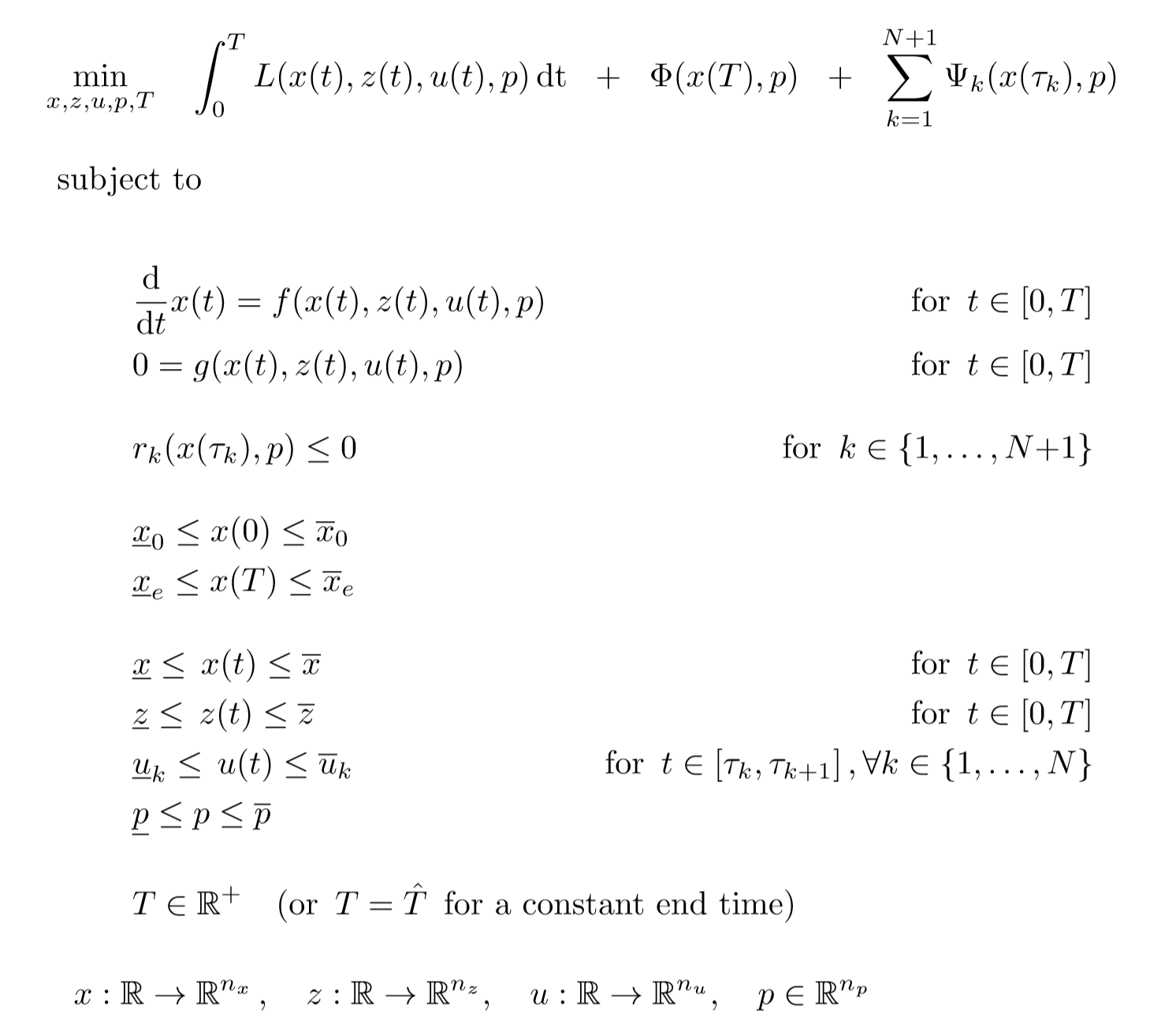where $x(t)$ is the state trajectory, $u(t)$ the control trajectory, $z(t)$ the algebraic state trajectory, $p$ the parameters, $L(x,z,u,p)$ the path cost function, $\Phi(x,p)$ the terminal cost function, $\Psi_k(x,p)$ the grid-cost function, $f(x,z,u,p)$ the system dynamics function (differential equation), $g(x,z,u,p)$ the algebraic constraints function, $r_k(x,p)$ the grid-constraints function. Note that the control bounds can be specified of each control interval, $\underline{u}_k$, $\overline{u}_k$.

If no algebraic states $z$ are defined, the system is described by an ordinary differential equation. If algebraic states are defined, then the dynamics function $f(x,z,u,p)$ together with the algebraic constraints function $g(x,z,u,p)$ define the system dynamics as a differential algebraic equation in the semi-implicit form. To solve an optimal control problem, the index of the differential algebraic equation has to be smaller than or equal to one.

The dimension of the variables are: number of states $n_x$ , number of algebraic states $n_z$, number of controls $n_u$, number of parameters $n_p$.

Single stage optimal control problems are implemented using the class ocl.Problem.

Multi-stage optimal control problems

Multi-stage problems (also called multi-phase problems) allow you to define a different system dynamics function for each of the stages. This formulation also allows you to implement discrete events where a jump in the state trajectory happens.

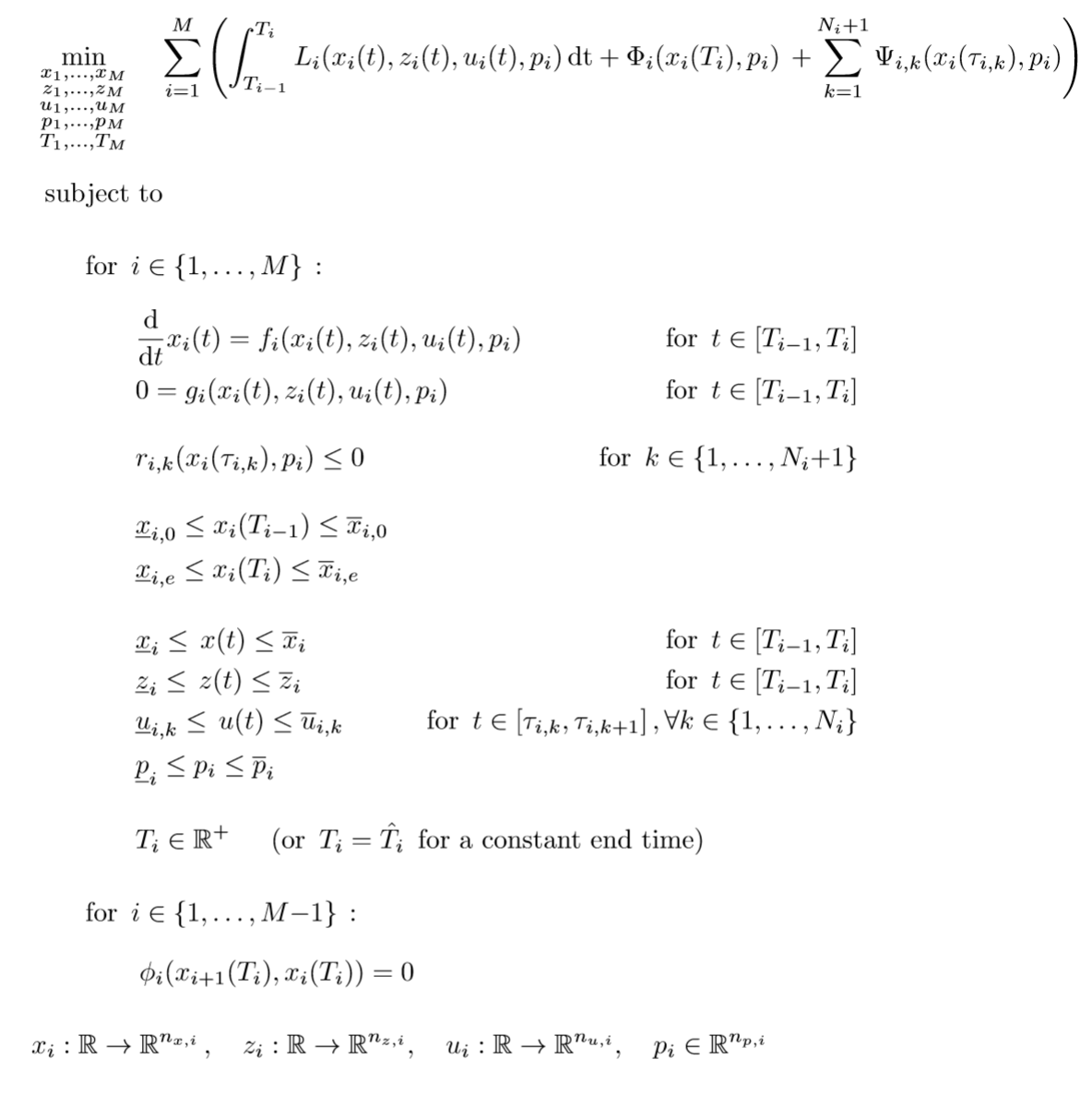
where $M$ is the number of stages, and $\phi_i$ is the stage transition function that relates the first state $x_{i+1}$ of stage $i{+}1$ to the last state $x_i$ of stage $i$ (at timepoint $T_i$).

All other functions and bounds can be specified for each stage as described above in the single-stage formulation. Stages are implemented using the class ocl.Stage, and the complete multi-stage problem can then be implemented using the class ocl.MultiStageProblem.

ocl.Constraint()

Methods

ocl.Cost()

Methods

ocl.DaeHandler()

Methods

ocl.MultiStageProblem(stages, transitions, userdata)

Arguments:

Returns:

Methods

ocl.Problem(T, vars, dae, pathcosts, gridcosts, gridconstraints, terminalcost, casadi_options, N, d, verbose, userdata, nlp_casadi_mx, controls_regularization, controls_regularization_value)

function vanderpol
  problem = ocl.Problem(10, @varsfun, @daefun, @pathcost, 'N', 30);

  problem.setInitialBounds('x',     0);
  problem.setInitialBounds('y',     1);

  problem.initialize('x', [0 1], [-0.2 -0.2]);

  [solution,timepoints] = problem.solve();

  % plotting of control and state p trajectory:
  ocl.plot(timepoints.controls, solution.controls.u)
  ocl.plot(timepoints.states, solution.states.p)
end

function varsfun(vh)
  vh.addState('x', 'lb', -0.25, 'ub', inf);
  vh.addState('y');
  vh.addControl('F', 'lb', -1, 'ub', 1);
end

function daefun(daeh,x,z,u,p)
  daeh.setODE('x', (1-x.y^2)*x.x - x.y + u.F);
  daeh.setODE('y', x.x);
end

function pathcost(ch,x,z,u,p)
  ch.add( x.x^2 );
  ch.add( x.y^2 );
  ch.add( u.F^2 );
end

Arguments:

Returns:

Methods

ocl.Simulator(vars, dae)

Arguments:

Returns:

Methods

ocl.Stage(T, vars, dae, pathcosts, gridcosts, gridconstraints, terminalcost, N, d, userdata)

stage = ocl.Stage([], @vars, @ode, 'N', 10, 'd', 2);

% Function definitions can be in the same file
% (if the main script is wrapped by a function)
% or in separate files:
function vars(sh)
  sh.addState('s');
  sh.addState('v');
end

function ode(sh,x,~,~,~)
  sh.setODE('s', x.v);
  sh.setODE('v', -10);
end

Arguments:

Methods

ocl.Variable()

% v is a solution of an OCP
% p=[px;py;pz] is of size 3x1
% p trajectory is of size 3x(N+1)
% F trajectory is of size 1xN
% with N control intervals
p = v.states.p;     % get state p trajectory
F = v.controls.F;   % get control F trajectory

% set all 3x1 p states to the same value
v.states.p = [3;2;1];
% set p states 4 and 5 in the trajectory
v.states.p(:,4:5) = [1,2,3;4,5,6].';

% set all px values of p in state trajectory
v.states.p(1,:) = 4;

% plotting of state p trajectory:
plot(t.states.value,v.states.p.value)

Methods

Variable:
  Size: [3681 1]
  Type: OclStructure
  Children: states, integrator, controls, parameters, time
  Value: [100;2;1;0;0;0;0;0;0;0;0;0;0;0;0..]

ocl.VarsHandler()

Methods

@(conh, k, K, x, p)

Arguments:

@(costh, k, K, x, p)

Arguments:

@(costh, x, z, u, p)

Arguments:

@(daeh, x, z, u, p)

Arguments:

@(vh)

Arguments:

CasadiOptions()

casadi_options = struct;
casadi_options.ipopt = struct;
casadi_options.ipopt.linear_solver = 'mumps';
casadi_options.ipopt.hessian_approximation = 'exact';

Returns: